In this blog, we will learn about IP addresses and netmasks.
IP
The Internet Protocol (IP) is a unique identifier for your device, similar to how a mobile number uniquely identifies your phone.
IP addresses are typically represented as four Octets for IPv4, with each octet being One byte/Octets in size, and eight octets for IPv6, with each octet being two bytes/Octets in size.
Examples:
IPv4: 192.168.43.64
IPv6: 2001:db8:3333:4444:5555:6666:7777:8888
For the purposes of this discussion, we will focus on IPv4.
Do we really require four Octets structure with dots between them?
The answer is NO
The only requirement for an IPv4 address is that it must be 4 bytes in size. However, it does not have to be written as four octets or even with dots separating them.
Let’s test this by fetching Google’s IP address using the nslookup command.
Convert this to binary number using bc calculator in Bash shell.
And you can see it’s working.
This is because the octet structure and the dots between them are only for human readability. Computers do not interpret dots; they just need an IP address that is 4 bytes in size, and that’s it.
The range for IPv4 addresses is from 0.0.0.0 to 255.255.255.255.
Types of IP Addresses
IP addresses are classified into two main types: Public IPs and Private IPs.
Private IP addresses are used for communication between local devices without connecting to the Internet. They are free to use and secure to use.
You can find your private IP address by using the ifconfig command
The private IP address ranges are as follows:
10.0.0.0 to 10.255.255.255 172.16.0.0 to 172.31.255.255 192.168.0.0 to 192.168.255.255
Public IP addresses are Internet-facing addresses provided by an Internet Service Provider (ISP). These addresses are used to access the internet and are not free.
By default
Private IP to Private IP communication is possible. Public IP to Public IP communication is possible.
However:
Public IP to Private IP communication is not possible. Private IP to Public IP communication is not possible.
Nevertheless, these types of communication can occur through Network Address Translation (NAT), which is typically used by your home router. This is why you can access the Internet even with a private IP address.
Netmasks Netmasks are used to define the range of IP addresses within a network.
Which means,
You can see 24 Ones and 8 Zeros.
Here, we have converted 255 to binary using division method.
255 ÷ 2 = 127 remainder 1
127 ÷ 2 = 63 remainder 1
63 ÷ 2 = 31 remainder 1
31 ÷ 2 = 15 remainder 1
15 ÷ 2 = 7 remainder 1
7 ÷ 2 = 3 remainder 1
3 ÷ 2 = 1 remainder 1
1 ÷ 2 = 0 remainder 1
So, binary value of 255 is 11111111
By using this, we can able to find the number of IP addresses and its range.
Since we have 8 zeros, so
Number of IPs = 2 ^8 which equals to 256 IPs. SO, the usable IP range is 10.4.3.1 – 10.4.3.254 and the broadcast IP is 10.4.3.255.
And we can also write this as 255.255.255.0/24 . Here 24 denotes CIDR (Classless Inter-Domain Routing).
Thats it.
Kindly let me know in comments if you are any queries in these topics.
This blog is about my experience of the Bio-diversity walk at Jallipatti which is located south of Udumalpet with a distance of 12km.
Table of contents
Bio-diversity walk introduction
Antlion
Social Spider
Cochineal
Sunai
Conclusion
Let’s understand the Bio-diversity walk.
Bio-diversity walk in which we observe the surroundings that not only consist of human beings but also plants, water resources, animals, birds, and micro-organisms which also have an equal right to live on this earth and own it.
We normally called these Flora and Fauna, Flora refers to all plant lives and fauna refers to all animal and bird lives.
And it does not end with observation but also tries to understand its characteristics, and its impact on the food chain, climate change, etc, and passes this information to the general public.
Bio-diversity walk enables us to understand the importance and impact of this flora and fauna.
We have chosen Jallipatti Karadu, it is a small hill slope that has a nice climate and has bio-diversity species in it.
We reached this place at 6.30am and started to climb along with Vetri, a schoolboy who is interested in exploring nature, and Mukesh, my school friend who runs the youth group named “Eegai Kulu” in Kuralkuttai village which focused on seed conservation, Grama sabha awareness, Biodiversity conservation, Bird survey and Insect survey.
He is the coordinator for this walk.
In this walk, we explored the varieties of Flora and Fauna. Mukesh and Vetri explained its characteristics since they have more experience in this field.
Mostly they will explain the flora and fauna species and if they don’t know, then we will take a species photo and upload it on INaturalist and E-Bird app in which the researchers are there, they will reply back with the characteristics and scientific names of those species.
Note: I have attached a Wikipedia link to the species image. Kindly click the image to see more details about these species.
Antlion
The first thing I learned in this Bio-diversity walk is Kulinari (Antlion), in which Kuli refers to the hole and Nari refers to Jackal which is meant for intelligent pranksters.
The Antlion
The Antlion is called a Jackal because of its intelligent method of capturing its prey by digging funnel-shaped pits in loose material with a soft layer so that if prey falls in the hole, it can’t escape it.
The Antlion further developed as an insect same as alike Dragonfly.
Social Spider
The next thing I had learned is the Social spider.
Usually, we have seen a spider in our homes which builds a web and it is seen as a solo player.
But, there are spiders who live in groups called colonies. It surprised me.
Here, the spiders used the prey not only for consumption but also for strengthening and maintenance of webs.
These webs were too sticky and even I forced hard to remove them from my cap(My cap got the web when I try to take the photo on another Flora).
Cochineal
It is an insect covered by a white layer (marked in a red circle) which is traditionally used for coloringfabrics in the olden days.
We tried to find out the color by pressing and we got Maroonish violet. In theolder days, people used to carry these groups of insects and made them dry by exposing them to sunlight. Once it gets dry, they will grind it to make colors.
After observing all of this, we have reached the top of the slope, there we viewed the Thirumoorthi dam and the ambiance is so good. Peaceful place with cold and heavy winds(my cap got wings to fly).
Sunai
We also found “Sunai” which is the water body in the rock that won’t dry. We have found out that the frogs in it.
Also, we have seen monkeys(grey langur) in which its body is grey with black face. I have seen this on the Discovery channel so far.
After all of this, we sat on the rock which have a better view of Thirumoorthi dam and the border spotted between the reserve forest and revenue forest.
Vetri brings snacks and we discussed the bio-diversity of that place and shared our own opinions.
Then the time is 10.30am. It’s hard to leave this beautiful place. When we stepped down the slope, we have seen the Eagle.
It’s surprising because earlier we had seen a flying Eagle. But this Eagle is flying but it doesn’t move forward or backward. It simply resists the wind against it and stands in the sky.
May be because it spots the prey, or it is gaining the energy to fly upwards.
Within 30 minutes, we stepped down the hill slope with so many memories.
Conclusion
To conclude, this Bio-Diversity walk was about knowledge transfer and opinion sharing in a peaceful environment with an awesome climate and with our beloved flora and fauna friends.
Thanks, Mukesh for introducing this awesome location, and the photos credit goes to him.
Thank you, everyone, for patiently reading this blog.
In this blog, we are going to see how to increase or decrease the size of the static partition in Linux without compromising any data loss and how to do that in Online mode without unmounting.
I already explained the basic concepts of partition in very detail in my previous blog. You can refer to that blog by clicking here.
In this practical, the Oracle VirtualBox is used for hosting the Redhat Enterprise Linux (RHEL8) Virtual Machine (VM).
The first step is to attach one hard disk. So, I attached one virtual hard disk with the size of 40GiB. That disk is named “/dev/sdc”. You can check the disk name and all other disks present in your VM by running the following command.
fdisk -l
Then, we have to do partition by using “fdisk” command.
fdisk /dev/sdc
Then, enter “n” in order to create a new partition. Then enter the partition number and specify the number of sectors or GiB. Here, we entered 20 GiB in order to utilize that much storage unless we do partition, we can’t utilize any storage.
We had created one partition named as “/dev/sdc1”. Next step is to format the partition. Here, we used Ext4 filesystem(format) to create an inode table.
Next step is to create one directory using “mkdir” command and mount that partition in that directory since we can’t directly use the hardware device no matter it is either real or virtual.
One file should be created inside that directory in order to check the data loss after Live scaling of static partition.
Ok, now the size of the static partition is 20 GiB, we are going to do scaling up to 30GiB without unmounting the partition. For this, again we have to run the following command.
fdisk /dev/sdc
Then delete the partition. Don’t bother about the data, it won’t lose.
Then enter “n” to create the new partition and specify your desired size. Here, I like to scale up to 30GiB. And then one warning will come and it says that “Partition 1 contains an ext4 signature” and ask us what to do with that either remove the signature or retain.
If you don’t want to lose the data, then enter “N”. Then enter “w” to save the partition. you can verify your partition size by running “fdisk -l” command in terminal. Finally, you increased the size of static partition.
First part is done. Then next step is to format the partition in order to create the file system. But this time, we will not use “mkfs” command, since it will delete all the data. We don’t need it. We have to do format without comprising the data. For that we have to run the following command.
resize2fs /dev/sdc1
Finally, we done format without comprising the data. We can check this by going inside that mount point and check whether the data is here or not.
Yes, data is here. It is not lost even though we created new partition and formatted the partition.
Live Linux Static Partition scaling without any data loss
In this blog, we are going to see how to increase or decrease the size of the static partition in Linux without compromising any data loss and done in Online mode.
I already explained the basic concepts of partition in very detail in my previous blog. You can refer to that blog by clicking here.
In this practical, the Oracle VirtualBox is used for hosting the Redhat Enterprise Linux (RHEL8) Virtual Machine (VM).
The first step is to attach one hard disk. So, I attached one virtual hard disk with the size of 40GiB. That disk is named “/dev/sdc”. You can check the disk name and all other disks present in your VM by running the following command.
fdisk -l
Then, we have to do partition by using “fdisk” command.
fdisk /dev/sdc
Then, enter “n” in order to create a new partition. Then enter the partition number and specify the number of sectors or GiB. Here, we entered 20 GiB in order to utilize that much storage unless we do partition, we can’t utilize any storage.
We had created one partition named as “/dev/sdc1”. Next step is to format the partition. Here, we used Ext4 filesystem(format) to create an inode table.
Next step is to create one directory using “mkdir” command and mount that partition in that directory since we can’t directly use the hardware device no matter it is either real or virtual.
One file should be created inside that directory in order to check the data loss after Live scaling of static partition.
Ok, now the size of the static partition is 20 GiB, we are going to do scaling up to 30GiB without unmounting the partition. For this, again we have to run the following command.
fdisk /dev/sdc
Then delete the partition. Don’t bother about the data, it won’t lose.
Then enter “n” to create the new partition and specify your desired size. Here, I like to scale up to 30GiB. And then one warning will come and it says that “Partition 1 contains an ext4 signature” and ask us what to do with that either remove the signature or retain.
If you don’t want to lose the data, then enter “N”. Then enter “w” to save the partition. you can verify your partition size by running “fdisk -l” command in terminal. Finally, you increased the size of static partition.
First part is done. Then next step is to format the partition in order to create the file system. But this time, we will not use “mkfs” command, since it will delete all the data. We don’t need it. We have to do format without comprising the data. For that we have to run the following command.
resize2fs /dev/sdc1
Finally, we done format without comprising the data. We can check this by going inside that mount point and check whether the data is here or not.
Yes, data is here. It is not lost even though we created new partition and formatted the partition.
Reduce the size of the Static Partition
You can also reduce the Static Partition size. For this, you have to follow the below steps.
Unmount
Cleaning bad sectors
Format
Mount
First step is to unmount your mount point since it is online, somebody will using it.
umount /partition1
Then we have to clean the bad sectors by running the following command
e2fsck -f /dev/sdc1
Then we have to format the size you want. Here we want only 20 GiB and we will reduce the remaining 10 GiB space. This is done by running following command.
resize2fs /dev/sdc1 20G
Then we have to mount the partition.
Finally, we reduced the static partition size.
Above figure shows that Data is also not lost during scaling down.
Thank you all for your reads. Stay tuned for my next article, because it is Endless.
Hosting your own WordPress website is interesting right!! Ok, come on let’s do it!!
We are going to do this practical from Scratch. From the Creation of our Own VPC, Subnets, Internet Gateway, Route tables to Deployment of WordPress.
Here, we are going to use Amazon Web Service’s RDS service for hosting our own WordPress site. Before that, let’s take a look at a basic introduction to RDS service.
Amazon Relational Database Service is a distributed relational database service by Amazon Web Services (AWS). It is a web service running in the cloud designed to simplify the setup, operation, and scaling of a relational database for use in applications. Administration processes like patching the database software, backing up databases and enabling point-in-time recovery are managed automatically.
Features of AWS RDS
Lower administrative burden. Easy to use
Performance. General Purpose (SSD) Storage
Scalability. Push-button compute scaling
Availability and durability. Automated backups
Security. Encryption at rest and in transit
Manageability. Monitoring and metrics
Cost-effectiveness. Pay only for what you use
Ok, let’s jump onto the practical part!!
We will do this practical from scratch. Since it will be big, so we divided this into 5 small parts namely
Creating a MySQL database with RDS
Creating an EC2 instance
Configuring your RDS database
Configuring WordPress on EC2
Deployment of WordPress website
Creating a MySQL database with RDS
Before that, we have to do two pre-works namely the Creation of Virtual Private Cloud(VPC), Subnets and Security groups. These are more important because in order to have a reliable connection between WordPress and MySQL database, they should be located in the same VPC and should have the same Security Group.
Since Instances are launched on Subnets only, Moreover RDS will launch your MySQL database in EC2 instance only that we cannot able to see since it is fully managed by AWS.
VPC Dashboard
We are going to create our own VPC. For that, we have to specify IP range and CIDR. We specified IP and CIDR as 192.168.0.0/16.
What is CIDR?. I explained this in my previous blog in very detail. You can refer here.
Lets come to the point. After specifying the IP range and CIDR, enter your VPC name.
Now, VPC is successfully created with our specified details.
Next step is to launch the subnet in the above VPC.
Subnet Dashboard
For Creating Subnets, you have to specify which VPC the lab should launch. We already have our own VPC named “myvpc123”.
And then we have to specify the range of Subnet IP and CIDR. Please note that the Subnet range should come under VPC range, it should not exceedVPC range.
For achieving the property of High Availability, We have to launch minimum two subnets, so that Amazon RDS will launch its database in two subnets, if one subnet collapsed means, it won’t cause any trouble.
Now, two Subnets with their specified range of IPs and CIDR are launched successfully inside our own VPC and they are available.
Next step is to create a security group in order to secure the WordPress and MySQL databases. Note that both should have the same Security Group or else it won’t connect.
For creating a Security Group, we have to specify which VPC it should be launched and adding a Description is mandatory.
Then we have to specify inbound rules, for making this practical simple, we are allowing all traffic to access our instance.
Now, the Security Group is successfully created with our specified details.
Now let’s jump into part 1 which is about Creating a MySQL database with RDS.
RDS dashboard
Select Create database, then select Standard create and specify the database type.
Then you have to specify the Version. Version plays a major role in MySQL when integrating with WordPress, so select the compactible version or else it will cause serious trouble at the end. Then select the template, here we are using Free-tier since it won’t be chargeable.
Then you have to specify the credentials such as Database Instance name, Master username and Master password.
Most important part is a selection of VPC, you should select the same VPC where you will launch your EC2 instance for your WordPress and we can’t modify the VPC once the database is created. Then select the Public access as No for providing more security to our database. Now, the people outside of your VPC can’t connect to your database.
Then you have to specify the security group for your database. Note that the Security Group for your database and WordPress should be the same or else it will cause serious trouble.
Note that Security Groups is created per VPC. After selecting Security Group, then click Ok to create the RDS database.
Creating an EC2 instance
Before creating an instance, there should be two things you configured namely Internet Gateway and Route tables. It is used for providing outside internet connectivity to an instance launched in the subnet.
Internet Gateway Dashboard
Internet Gateway is created per VPC. First, we have to create one new Internet Gateway with the specified details.
Then you have to attach Internet Gateway to the VPC
Next step is to create Routing tables. Note that Route table is created per Subnet.
We have to specify which VPC in which your subnet is available to attach routing table with it, specify Name and click create to create the route table.
Then click Edit route to edit the route details namely destination and target. Enter destination as 0.0.0.0/0 for accessing any IP anywhere on the Internet and target is your Internet Gateway.
After entering the details, click Save routes.
We created a Route table, then we have to attach that table to your Subnet. For that click Edit route table association and select your subnet where you want to attach the route table with it.
Now, lets jump into the task of creating an EC2 instance.
First, you have to choose the AMI image in which you used for creating an EC2 instance, here I selected Amazon Linux 2 AMI for that.
Then you have to select Instance type, here I selected t2.micro since it comes under free tier.
Then you have to specify the VPC,Subnet for your instance and you have to enable Auto-assign Public IP in order to get your Public IP to your instance.
Then you have to add storage for your instance. It is optional only.
Then you have to specify the tags which will be more useful especially for automation.
Then you have to select the Security Group for your instance. It should be the same as your database have.
And click Review and Launch. Then you have to add Keypair to launch your EC2 instance. If you didn’t have Keypair means, you can create at that time.
Configuring your RDS database
At this point, you have created an RDS database and an EC2 instance. Now, we will configure the RDS database to allow access to specific entities.
You have to run the below command in your EC2 instance in order to establish the connection with your database.
export MYSQL_HOST=<your-endpoint>
You can find your endpoint by clicking database in the RDS dashboard. Then you have to run the following command.
mysql --user=<user> --password=<password> dbname
This output shows the database is successfully connected to an EC2 instance.
In the MySQL command terminal, you have to run the following commands in order to get all privileges to your account.
CREATE USER 'vishnu' IDENTIFIED BY 'vishnupassword';
GRANT ALL PRIVILEGES ON dbname.* TO vishnu;
FLUSH PRIVILEGES;
Exit
Configuring WordPress on EC2
For Configuring WordPress on EC2 instance, the first step is to configure the webserver, here I am using Apache webserver. For that, you have to run the following commands.
sudo yum install -y httpd
sudo service httpd start
Next step would be download the WordPress application from the internet by using wget command. Run the following code to download the WordPress application.
wget https://wordpress.org/latest.tar.gz
tar -xzf latest.tar.gz
Then we have to do some configuration, for this follow the below steps.
cd wordpress
cp wp-config-sample.php wp-config.php
cd wp-config.php
Go inside the wp-config.php file and enter your credentials (including your password too)
Then, Goto thislinkand copy all and paste it to replace the existing lines of code.
Next step is to deploy the WordPress application. For that, you have to run the following commands in order to solve the dependencies and deployWordPress in the webserver.
In this, Netmask 255.255.255.248 denotes the IP range which have the connection between them.
If you convert to binary form means, it looks like this.
11111111 11111111 11111111 11111000
For the last three places(where the zeros located), we can accommodate 8 combinations. So it decided the number of IPs (IP range) that can connect each other.
The range of IPs are that can connect each other is 162.168.1.0–162.168.1.7.
So in this way, System A can ping to System B (162.168.1.2) and System C (162.168.1.4).
If you convert to binary form means, it looks like this.
11111111 11111111 11111111 11111110
For the last one place(where the zero located), we can accommodate 2 combinations. So it decided the number of IPs (IP range) that can connect each other.
So the range of IPs that are connected to each other are two in numbers namely 168.162.1.0 and 162.168.1.1.
In this way System B can ping to System A. It is noted that IP of System C (162.168.1.4) is not in range, that’s the reason for not ping.
Finally, if you take a look on routing rule in System C.
Here, the Netmask specified is 255.255.255.254. So the last one place(where the zero located), we can accommodate 2 combinations. So it decided the number of IPs (IP range) that can connect each other.
So the range of IPs that are connected to each other are two in numbers namely 168.162.1.0 and 162.168.1.1.
In this way, System C can ping to System A. It is noted that IP of B(162.168.1.2) is not in range, that’s the reason for not ping.
Thank you for your reads. Stay tuned for my next article.
The first question that arise on your mind after seeing this title is “Why I want to block Facebook? What is the need for this?”. The answer for your question is may be you have kids in your home or they may be lying you by saying they are attending online class but actually they are wasting their precious time in Social Networks. It is more common nowadays since this Pandemic happened.
Ok. Lets come to the point.
Here we are going to see how to block Facebook but ensure the access to Google in the same system. May be you had seen this setup in your college systems where we are not allowed to use some kind of the websites.
But before this you should know some basic Linux Networking concepts and terminologies.
Note: Here I am using Redhat Enterprise Linux (RHEL8) which is hosting by Oracle VirtualBox.
IP address
In simple words, it is like your mobile number which is used for identified you uniquely. Every computer have their unique IP address. IP stands for “Internet Protocol”, which is the set of rules governing the format of data sent via the internet or local network.
IP addresses are not random. They are mathematically produced and allocated by the Internet Assigned Numbers Authority (IANA), a division of the Internet Corporation for Assigned Names and Numbers (ICANN). ICANN is a non-profit organization that was established in the United States in 1998 to help maintain the security of the internet and allow it to be usable by all. Each time anyone registers a domain on the internet, they go through a domain name registrar, who pays a small fee to ICANN to register the domain.
IP address is of two types based on the number of octates namely IPv4 and IPv6.
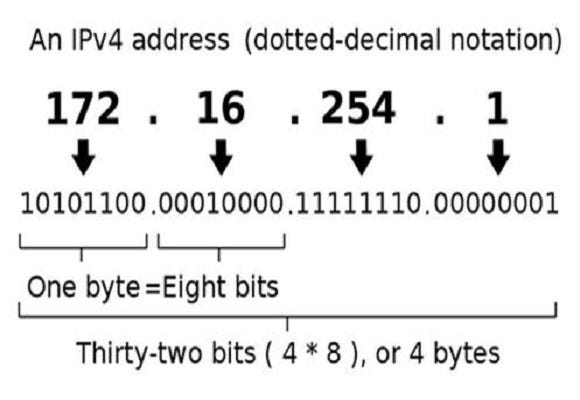
IPv4
IPv4
After figure clearly explains about IPv4. Its size is 32 bits or 4 bytes. Each number in the set can range from 0 to 255. So, the full IP addressing range goes from 0.0.0.0 to 255.255.255.255. That means it can provide support for 2³² IP addresses in total around 4.29 billion. That may seem like a lot, but all 4.29 billion IP addresses have now been assigned, leading to the address shortage issues we face today.
IPv6
IPv6
IPv6 utilizes 128-bit Internet addresses. Therefore, it can support 2¹²⁸ Internet addresses — 340,282,366,920,938,463,463,374,607,431,768,211,456 of them to be exact. The number of IPv6 addresses is 1028 times larger than the number of IPv4 addresses. So there are more than enough IPv6 addresses to allow for Internet devices to expand for a very long time.
We can find your system IP address in RHEL8 by using the following command.
ifconfig enp0s3
RHEL8
Here our IPv4 address is 192.168.43.97 and IPv6 address is fe80::ad91:551e:e05a:5ab8.
Netmask
Netmask plays a major role in finding the range of IPs in which they can ping each other. It has two parts namely Network ID and Host ID
For example, with an IP address of 192.168.100.1 and a subnet mask of 255.255.255.0, the network ID is 192.168.100.0 and the host ID is 1. With an IP of 192.168.100.1 and a subnet mask of 255.0.0.0, the network ID is 192 and the host ID is 168.100.1
Netmask
In the above example, NetMask is 255.255.255.0 and if we convert host ID into binary, it has 8 zeros. 2⁸ =256 IPs available to connect.
CIDR
Classless Inter-Domain Routing, or CIDR, was developed as an alternative to traditional subnetting. The idea is that you can add a specification in the IP address itself as to the number of significant bits that make up the routing or networking portion.
CIDR notation
For example, we could express the idea that the IP address 192.168.0.15 is associated with the netmask 255.255.255.0 by using the CIDR notation of 192.168.0.15/24. This means that the first 24 bits of the IP address given are considered significant for the network routing.
In simple words, CIDR is number of Ones in Netmask.
Gateway
A gateway is a router that provides access for IP packets into and/or out of the local network. The term “default gateway” is used to mean the router on your LAN which has the responsibility of being the first point of contact for traffic to computers outside the LAN.
The default gateway IP can be found by using the following command on RHEL8.
route -n
Here, in routing table ,the Gateway IP is 192.168.43.146. The Destination IP mentioned 0.0.0.0 indicates that we can go anywhere on Internet and accessing any websites without any restriction.
Here comes the practical part.
First we have to delete the rule which permits user to access any kind of websites. It is done by running following command.
route del -n 0.0.0.0 netmask 0.0.0.0 gw 192.168.43.146 enp0s3
After this, if you want to ping google or facebook, it wont possible
For now, even if you are having internet connection, you feels like you are in offline because your system doesn’t know the gateway address, so impossible to go out.
For this, you have to add one rule to your IP table for granting access to Google only. It is done by below command.
You can find Google IP for your PC by running the below command.
nslookup google.com
After run these command, you can notice that your Facebook IP is not pinging and at the same time your Google IP is pinging and you have good connectivity with Google.
Thank you all for reads. Hope you enjoyed this article. Stay tuned for my next article.
A web application is application software that runs on a web server, unlike computer-based software programs that are run locally on the operating system of the device.
For the Web app, it needs an environment that cannot be compromised. In this article, we are going to see how to create an environment for running a Webapp in Container with Virtual Machine as a host. Here we used Oracle VirtualBox’s RHEL8 Virtual Machine is acting as a host.
Contents:
Docker Installation
Configuration of HTTP Server
Python Interpreter setup
Docker Installation
Docker is a set of platform as a service products that use OS-level virtualization to deliver software in packages called containers. Containers are isolated from one another and bundle their own software, libraries and configuration files; they can communicate with each other through well-defined channels. The installation consists of below steps.
Yum Configuration
Service Installation
Starting Service
Permanently Enabling
Yum Configuration
First step is to configure the yum so that we can configure Docker.
Second step is to install the Docker by using the command given below.
dnf install docker-ce --nobest
Third step is to start the service.
systemctl start docker
Then we have to make this service permanent after every reboot.
systemctl enable docker
Then you have to launch the container, but launching container needs Docker images. Here, we will use Centos image. We will download the image using the command shown below.
docker pull centos
Then we have to launch the container by using below command.
docker run -it --name mycentos -p 1234:80 centos
After running this command, we will go inside the container. You can verify it by seeing the change in hostname.
Configuring HTTP Server
Configuration inside docker container requires three steps namely Installing Package, Start the service and Make it Permanent.
You can install the HTTP server by using yum.
yum install httpd -y
Then you have to start the server inside the container by using the command shown below.
/usr/sbin/httpd
Then you have to make this service permanent by copying “/usr/sbin/httpd” inside the /etc/.bashrc file.
Python Interpreter setup
Final step is to setup the Python interpreter, because we can create a webapp using Python. You can install this setup by running the command shown below.
yum install python3 -y
Now, the complete environment is ready to create a webapp.
Nowadays, data are generated and updated per second. In this Big data world, Some times We can’t even predict how much data we will get in the future. For storing these massive amounts of data, typically we are using Clustering technologies, so such technique is Hadoop Distributed File System (HDFS). Hadoop is an open-source Java-based framework used for storing data and running applications on clusters of commodity hardware.
Since the size of data is exponentially growing, to store these data efficiently and effectively, storage should possess some special characteristics in nature namely Dynamic Storage.
In this article, we are going to see how to set up a Dynamic Storage unit to the Data node in HDFS Cluster.
For those who are not familiar with Hadoop and HDFS cluster, I have already written some articles. You can find them in my profile.
To setting up a Dynamic Storage unit in HDFS Cluster, we use one important concept in Linux. Yes, it is none other than LVM.
In Linux, Logical Volume Manager (LVM) is a device mapper framework that provides logical volume management for the Linux kernel. Most modern Linux distributions are LVM-aware to the point of being able to have their root file systems on a logical volume.
OK, let’s go step by step. In this practical, I used Redhat Enterprise Linux (RHEL8) OS and Oracle VM VirtualBox which is cross-platform virtualization software that allows users to extend their existing computer to run multiple operating systems at the same time.
Step 1: Creation of new hard disk
We can’t increase the storage with the existing amount of storage in hand. So We have to create additional storage. For this, Oracle Virtualbox provided one feature namely Virtual Hard disk which looks the same as a real hard disk but it is not. I already created two Virtual hard disks which shown below.
I am clearly explained step by step about creating a virtual hard disk in my previous article. You can find this by clicking here.
You can also verify whether the hard disk is there or not by running the following command in the command line.
fdisk -l
In the above image, you can find our newly created virtual hard disk namely /dev/sdb and /dev/sdc which has a size of 50 GiB and 40 GiB.
Step 2: Creation of LVM
The creation of LVM involves the following steps namely
Creation of Physical Volumes (PV)
Creation of Volume Groups (VG)
Creation of Logical Volumes (LV)
Logical Volume formatting
Mounting Logical Volumes
Creation of Physical Volumes
We have to run “pvcreate” command to initialize a block device to be used as a physical volume.
The following command initializes /dev/sdband /dev/sdcas LVM physical volumes for later use as part of LVM logical volumes. You can view the Physical volumes by running pvdisplay command.
In future, if you want to remove the physical volumes, you have to run the following command.
pvremove diskname
Creation of Volume Groups (VG)
To create a volume group from one or more physical volumes, use the vgcreate command. The vgcreate command creates a new volume group by name and adds at least one physical volume to it.
vgcreate myvg /dev/sdb /dev/sdc
The above commands created one Volume Group named “myvg” which comprises of /dev/sdb and /dev/sdc volumes. You can also view the further details by using vgdisplay vgnamecommand.
By default, the block size of Volume Groups is fixed as 4MiB but we can change according to our requirements.
In the future, if you want to remove the Physical Volumes from a Volume Group, you have to run the following command
vgreduce vgname pvname
Creation of Logical Volumes (LV)
We can create the Logical volume by using lvcreate command. We can also create one Logical volume with 88% of the total size of Volume Groups. When you create a logical volume, the logical volume is carved from a volume group using the free extents on the physical volumes that make up the volume group.
Here, we created one Logical Volume named “mylv1” with the size of “myvg” size.
You can also view the further details of the logical volume by running lvdisplay command.
Normally logical volumes use up any space available on the underlying physical volumes on a next-free basis. Modifying the logical volume frees and reallocates space in the physical volumes.
Format
If you take any hard disk, without done formatting, we can’t use that space even it has free space. The format is also known as Filesystem, which has an Inode table that acts as an Index table for OS operations. Here, the format is ext4.
mkfs.ext4 /dev/myvg/mylv1
Mount
It is not possible to use the physical device directly. You have to mount to one folder to use.
mount /dev/myvg/mylv1 /lvm2
We mounted that Logical Volume into one directory named “lvm2“.
You can view this mount by running df -hT .
Step 3: HDFS Cluster Configuration
We already discussed this configuration in my previous article. You can check this by clicking here.
Then we have to update this directory name in datanode’s hdfs-site.xml file.
Then start the name node and data node.
Step 4: Increase the size of the data node
We know that 10GiB space is available in our Volume group. We can utilize that space to increase the size of the data node in the HDFS Cluster.
Steps:
lvextend
format
mount
We have to extend the Logical volume size by using lvextend command.
lvextend --size +5G /dev/myvg/mylv1
We extended logical volume by an extra 5GiB.
Then we have to format the remaining space (5GiB) by using resize2fs command because format command will format the total hard disk again, so there will be a data loss.
resize2fs /dev/vgname/lvname
The size of data node is increased by 5GiB.
Reduce the size of the Data node
You can also reduce the data node size. For this, you have to follow the below steps.
Unmount
Cleaning bad sectors
Format
Lvreduce
Mount
First step is to unmount your mount point since it is online, somebody will using it. But before that you have to stop data node because it is busy.
Then we have to clean the bad sectors by running the following command
e2fsck -f /dev/mapper/vgname-lvname
Then we have to format the size you want. Here we want only 50GiB and we will reduce the remaining 5GiB space. This is done by running following command.
resize2fs /dev/mapper/vgname-lvname 50G
Then we have to reduce the 5GiB space by using lvreduce command.
lvreduce -f --size 50G /dev/mapper/vgname-lvname
Then start the data node in HDFS Cluster.
Finally, we reduced the data node size.
Thank you all for your reads. This article explaining the manual method for providing the Elasticity to data node in HDFS cluster. The Next article will be how to do these using Automated Python Scripts. Stay tuned.Will see you all in my next article. Have a good day.
In this article, we are going to see about what is the Content Delivery Network, why we need them, what are its use cases and then finally we are going to set up our own Content Delivery Network with Fast, Secure and high availability using one of the most powerful services provided by AWS namely Cloudfront.
Content Delivery Network
A Content Delivery Network (CDN) is a globally distributed network of web servers whose purpose is to provide faster content delivery. The content is replicated and stored throughout the CDN so the user can access the data that is stored at a location that is geographically closest to the user.
This is different and more efficient than the traditional method of storing content on just one, central server. A client accesses a copy of the data near to the client, as opposed to all clients accessing the same central server, in order to avoid bottlenecks near that server.
source: Globaldots
High content loading speed ==positive User Experience
CDN Architecture model
The above figure clearly illustrates the typical CDN model. When a user requests the content, for the first time it will send to Content Provider, then Content Provider will send their copy of the document known as Source to CDN and that copy is stored as digital information which is created, licensed and ready for distribution to an End User. If the User requests the content again, he will receive the content from CDN only which is located nearer to the geographical location of the user, not from Content Provider. We can reduce latency and ensure high availability.
Benefits of CDN over Traditional method
CDN enables global reach
100% percent availability
Your reliability and response times get a huge boost
Decrease server load
Analytics
Use-Cases of CDN
Optimized file delivery for emerging startups
Fast and secure E-Commerce
Netflix-grade video streaming
Software Distribution, Game Delivery and IoT OTA
CloudFront
credits: whizlabs
Amazon CloudFront is a fast content delivery network (CDN) service that securely delivers data, videos, applications, and APIs to customers globally with low latency, high transfer speeds, all within a developer-friendly environment. CloudFront uses Origins from S3 for setting up its Content Delivery Network.
Cloudfront uses Edge locations to store the data cache. Currently, AWS now spans 77 Availability Zones within 24 geographic regions around the world and has announced plans for 18 more Availability Zones and 6 more AWS Regions in Australia, India, Indonesia, Japan, Spain, and Switzerland.
AWS uses DNS to find the nearest data centers for storing the caches. Data comes from Origin to Edge location and Edge location to our PC.
Practicals
Now I am going to show you how to setup your Custom Own Content Delivery Network for your content which includes images, videos, etc. Before going into this, please refer to my previous blog where I explained how to launch the instances, security groups, key-pairs, EBS volumes by using AWS Command Line Interface from scratch.
Click here to view my previous blog for getting started with AWS CLI if you not known already about AWS CLI.
Pre-requisites
AWS account
AWS instance
EBS volume
For saving time, I already launched one Amazon instance and one EBS volume sized 10GB and attached to its instance.
Steps
Installing HTTPD server
Making its document root persistent
S3
Deployed it to CloudFront
Installing HTTPD server
Since the package manager “YUM” is already installed in Amazon Linux 2, sorun the following commands for configuration of HTTPD server in that instance.
yum install httpd -y
Then we have to start the service.
yum start httpd
We have to enable the service. So that we need not start the service again and again after every reboot.
yum enable httpd
Making its document root persistent
Since the OS in Amazon 2 Linux is RHEL 8, so the document root of HTTPD server is /var/www/httpd. The document root is the location where the HTTPD server reads and deployed it into the web page. We have to make that document root persistent in order to secure the data from being lost due to OS crash etc.
For that, you have to ready with the previously created one EBS volume and done with the partition. Then run the following command.
mount /var/www/html /partition
Simple Storage Service
Since the Origin for CloudFront is S3, we have to setup S3 so that we can get the Origin Domain name for CloudFront. In S3, the folders are said to be buckets and files are said to be Objects.
First step is to create a bucket by using the following command syntax.
aws s3 mb s3://bucketname
The second step is to move/copy the objects to the buckets by using following command syntax.
aws s3 mv object-location s3://bucketname
By default, Public access for S3 buckets is blocked. We have to release the access by running the following command syntax in your Windows Command Prompt.
We had completed the S3 setup, the HTML code of the webpage is shown below.
CloudFront
source: stackflow
Since Origin S3 setup is over, now we have to setup the CloudFront by creating one distribution using Origin Domain Name from S3 and Object name as Default Root Object.
We have to run the following command to create a distribution
After creating the distribution, CloudFront will give one domain address, we have to copy that domain address to that HTML code and it will replace the S3 domain address.
Finally our Output will be…
Thank you friends for your patience to read this article. Kindly please let me know about your feedbacks so that I can improve my writings. I even didn’t need any claps or likes too. Just need feedback for improving me to give engaged insightful contents to you all. That’s it. Have a good day.
AWS Command Line Interface(AWS CLI) is a unified tool using which you can manage and monitor all your AWS services from a terminal session on your client.
Why AWS CLI?
Easy Installation: The installation of AWS Command Line Interface is quick, simple and standardized.
Saves Time: You need not log on to your account again and again for checking or updating the current status of services. Thus it saves time a lot
Automates Processes: AWS CLI gives you the ability to automate the entire process of controlling and managing AWS services through scripts. These scripts make it easy for users to fully automate cloud infrastructure.
Supports all Amazon Web Services: Prior to AWS CLI, users needed a dedicated CLI tool for just the EC2 service. But now AWS CLI lets you control all the services from one simple tool.
Objectives
Create a key pair.
Create a security group & its rules
Launch an instance using the above created key pair and security group.
Create an EBS volume of 1 GB.
The final step is to attach the above created EBS volume to the instance you created in the previous steps.
Pre-requisites
AWS CLI should be installed in your system
AWS IAM account with Administrator Access
Creation of Key-Pair:
A key pair, consisting of a private key and a public key, is a set of security credentials that you use to prove your identity when connecting to an instance. It is essential to launch an instance.
aws ec2 create-key-pair --key-name MyKeyPair
We can also verify this in AWS Management Console which is shown in below figure.
Creation of Security Group:
A security group acts as a virtual firewall for your instance to control inbound and outbound traffic. When you launch an instance in a VPC, you can assign up to five security groups to the instance.
Security groups act at the instance level, not the subnet level. Therefore, each instance in a subnet in your VPC can be assigned to a different set of security groups.
There are two types of traffics namely Inbound or Ingress and Outbound or Egress traffic. We have to frame the rules for these traffics. You can choose a common protocol, such as SSH (for a Linux instance), RDP (for a Windows instance), and HTTP and HTTPS to allow Internet traffic to reach your instance. You can also manually enter a custom port or port ranges.
Inbound traffic:
To allow inbound traffic entered to your instance, you have to create ingress rules. In this ssh and HTTP protocols are allowed by creating rules for them because our instance is mostly accessed by these types of protocols only by the clients.
To allow outbound traffic entered to your instance, you have to create egress rules. Normally, we can allow all protocols and ports so that our instance can have full outside accessibility.
aws ec2 authorize-security-group-egress --group-id sg-02658f46b1c47c775 --protocol all --cidr 0.0.0.0/24
Outbound rules
Creation of EC2 instances:
Amazon Elastic Compute Cloud (Amazon EC2) is a web service that provides secure, resizable compute capacity in the cloud. It is designed to make web-scale cloud computing easier for developers. For create an instance, two things required namely KeyPair and SecurityGroups which we already created in the previous steps.
Amazon Elastic Block Store (EBS) is an easy to use, high-performance block storage service designed for use with Amazon Elastic Compute Cloud (EC2) for both throughput and transaction-intensive workloads at any scale. It provides extra storage space to an instance. Scripts to create an EBS volume using AWS CLI is given below.
When the storage in EC2-instance is going to fully utilized, the extra EBS volume is required to store further data. For this, we have to create and attach EBS volume to an EC2-instance. For this, we have to specify the instance id and security group in the following command.
Finally our objective is successfully executed. This is only the start of AWS CLI, further the more to come in future. Feel free to express your views through feedbacks and if you have any doubts and need clarifications, you can contact me through linkedin
Hope the title makes some sense to you that what we are going to discuss. In this article, we will going to see this from scratch. Here, we use Linux partition concepts for limiting the size of the contribution of the data node. Why we need to limit the size, because we cant shut down the data node when it is exhausted and also limiting promotes dynamic storage.
Note:
In this task, the OS we used is Redhat Linux8 and you can use any Linux OS and it is installed on top of Oracle Virtualbox.
Pre-requisites:
Hadoop 1.2.1 should be installed in your system
Java jdk-8u171 should be installed in your system
Contents:
Hadoop
Linux partitions
Configuration of HDFS cluster
Hadoop
Apache Hadoop is an open-source framework which is used to store massive amount of data ranging from Kilobyte to Petabytes. It functions based on clustering of multiple computers by distributed storage instead of one single Large computer thus results in reduction of cost and time.
Linux partitions
In RHEL8 Linux, there are three types of partition namely Primary, Extended and Logical partition. Normally only the four partitions are possible per hard disk. Its because the metadata of partitions stored in 64 bytes only and size of metadata for one partition is 16 bytes. So we have to do some trick, we have to divide harddisk into two partitions namely three Primary partition and one Extended partition. In Extended partition, partition is considered as one new Hard disk thus we can perform this trick again to get more partitions.
Totally, we can create three Primary partitions, one extended partitions and Sixty Logical partitions. Totally 64 partitions can create and we can use 63 partitions.
Before creating partition, we required a raw hard disk. you can buy a new hard disk or create a Virtual hard disk in Oracle Virtualbox. Please follow the below steps to create a Virtual hard disk in RHEL8 using Oracle virtual box.
Open Settings in Oracle VirtualBox
2. Select Add hard disk in Controller: SATA menu
3. Select Create Disk Image icon
4. Select Virtual Disk Image option
5. Then select Dynamically allocated option in order to make storage Dynamically filled.
6. Give your required storage and then click Create button
7. Then attach the storage and click choose button
8. You can find your created storage details in your dashboard
Now we have a raw hard disk, in raw hard disk we can’t store any data. We have to do partition to utilize this hard disk.
Steps involved to create a partition:
Physical partition
Format
Mount
Physical partition:
We have to decide how much space we required for our partition. After that run
fdisk -l
to find out details of hard disk details.
You can find the hard disk named /dev/sdb which we previously created. Then execute the following command
fdisk /dev/sdb
and enter n for new partitions and enter p for primary partitions and select how many sectors or GB according to your required size and enter “w” to save. You can found these in below image.
Enter below command to check whether the partition was created or not
fdisk -l /dev/sdb
But we can create only 4 partitions, so we have to do some tricks. We can create 3 Primary partitions adn create one Extended partition for remaining size.
Extended partition is treated like a Hard disk, we can create Logical partitions inside Extended partition and Logical partition sector’s range will be same as range of Extended partition. You can seen this in below image.
Format:
First step is done. Then we have to format the disk. Format process is like creating an index in hard disk which is used by OS for searching a file and displayed to us when we click to open a file. Enter the following command for formatting the hard disk in ext4 format. You can use any format according to your requirements.
mkfs.ext4 /dev/sdb1
Mount:
Next step is to mount the hard disk in any of the folder/directory in OS. Because, we cant go inside or access the folder in hard disk, for this we have to link/mount this to OS folder. For this, we have to enter the following commands in Linux terminal. We created drive1 folder in root directory and its size is 1GB.
mount /dev/sdb1 /drive1
Configuring HDFS cluster
Hadoop works based on multiple clusters which comprises of three types of nodes namely Master node, Client node and Data node.
Master node
It stores the metadata of files stored in data node. It is used to provide the data node IPs to client and thereby it act as a connecting bridge between them.
Client node
This node is an End-user node that decides the number of replication blocks and block size. Risk factor plays a major role in deciding replication blocks. It is directly proportional to number of replication blocks. By default,the number of replication blocks is three which can be increased or decreased based on our applications.
Data node
It is also known as slave node which is used to store the data which is provided by client node.
These three nodes combined to form a Hadoop Distributed FileSystem (HDFS) cluster. But before configuring this cluster, we are going to see how to do partition in RHEL-8 Linux since it will help us to achieve our goal of limiting the size of contribution of data node to their master node.
Master node configuration:
This configuration involves two files namely hdfs-site.xml file which involves storage folder for metadata and core-site.xml for networking part.
HDFS-site.xml file
In core-site.xml file, we have to enter the IP as 0.0.0.0 in order to giving permissions to connect with any IP as a master node. we have to enter port number as 9001 since it is a default port numbe rfor Hadoop.
Core-site.xml file
Then w have to start namenode by using following command.
hadoop-daemon.sh start namenode
You can check whether the node is running or not by using Java Process(JPS)
Data node configuration:
It also involves two files namely hdfs-site.xml file which involves storage folder for metadata and core-site.xml for networking part.
hdfs-site.xml file
In core-site.xml file, we have to enter master IP in order to contribute your storage with it.
core-site.xml file
Then run the following commands to start a datanode
hadoop-daemon.sh start datanode
Finally, your data node is connected with master node and formed a HDFS-cluster and you can check this with a webGUI. For this you have to perform following commands in your browser.
https://masterip:50070
Finally we limited our storage to 1 GiB for datanode to namenode. You can see this in following picture.
Thank you for reading this article. Hope you got a clarity about setting HDFS cluster and Linux partitions. Please kindly share your views as a comments so that I can improvise myself to give you all a quality content.